Background
The Stroop effect is one of the most robust findings in psychological science. In a standard visual Stroop task, participants are presented a sequence of stimuli in the form of colourful words and are instructed to respond by naming the colour in which the given stimulus is presented. One stimulus-response pair is called a trial.
Study design
The present study investigated the visual Stroop effect. Participants were allocated into one of two conditions, either “congruent” or “incongruent”. Each participants was then presented with two blocks of trials. The first block – the “non-colour-word” block – the stimuli presented were not colour words. The task was to name the colour in which the stimuli are displayed as quickly and accurately as possible. The task looks something like this:
The second block – the “colour-word” block – differed based on the condition (group) to which the given participant was allocated. In the “congruent” condition, the stimuli were colour-words and the colour in which they were displayed agreed with the meaning of the word. Again, the task was to name the colour as quickly and accurately as possible. This is what the condition looks like:
In the “incongruent” condition, the colour in which the words were displayed was not the same as the meaning of the stimuli. The task was the same. This is what it looks like:
Reaction time on each trial was recorded in milliseconds as was whether or not participant’s response was correct. If no response was recorded within 3 seconds, an incorrect response was recorded and the next trial was presented.
You were called upon to analyse the data and decide whether or not there is a difference between reaction times on congruent vs incongruent trials. You should only consider correct responses on the colour-word trials, excluding any improbably fast responses (less than 200ms).
Data
The dataset is available at https://and.netlify.app/datasets/stroop.csv
Codebook
| Varaible name | Content | Notes |
|---|---|---|
id |
Unique participant number | |
block |
Non-colour-words (0) vs colour-words (1) | Within-subjects variable |
group |
Congruent (0) vs Incongruent condition | Between-groups variable |
trial |
Trial number | |
correct |
Correct (1) or incorrect (0) response on the trial | |
rt |
Reaction time in milliseconds |
Tasks
Drawing on the information above, complete the following tasks:
Setting up
Task 1
Create a new R Markdown document in your week_06 project folder.
Use a combination of code chunks with R code and body text to complete the remaining tasks.
Hypotheses
Task 2
Formulate the statistical null and alternative hypotheses.
\[H_0:\ ...\]
\[H_1:\ ...\]
\[H_0:\ \mu_{\text{congruent}} = \mu_{\text{incongruent}}\]
\[H_1:\ \mu_{\text{congruent}} \ne \mu_{\text{incongruent}}\]
Data inspection
Task 3
Read in the data.
stroop <- readr::read_csv("https://and.netlify.app/datasets/stroop.csv")
Task 4
Familiarise yourself with the data set.
Task 4.1
How many variables are there?
ncol(stroop)
[1] 6Task 4.2
Data from how many participants are included in the dataset?
There are many ways to do this:
Task 4.3
How many trials did each participant complete per block?
# A tibble: 232 x 3
# Groups: id [116]
id block n
<dbl> <dbl> <int>
1 1 0 40
2 1 1 40
3 2 0 40
4 2 1 40
5 3 0 40
6 3 1 40
7 4 0 40
8 4 1 40
9 5 0 40
10 5 1 40
# ... with 222 more rows## two more lines and you don't have to browse through the output
stroop %>%
  dplyr::group_by(id, block) %>%
dplyr::tally() %>%
dplyr::ungroup() %>%
dplyr::summarise(unique_n = unique(n))
# A tibble: 1 x 1
  unique_n
     <int>
1       40
Task 4.4
What proportion of trials were responded to incorrectly (including non-responses)?
From the description of the study design:
If no response was recorded within 3 seconds, an incorrect response was recorded and the next trial was presented.
If correct response is coded as 1 and incorrect as 0, then \(N - \sum{\text{correct}}\) gives the number of incorrect responses. Dividing this number by \(N\) gives proportion of incorrect responses.
Task 4.5
Assuming a trial automatically ends after 3 seconds, how many trials recorded no response?
This is a simple filtering task:
Data cleaning and wrangling
Task 5
Convert the block and group variables into factors and give them labels according to the codebook above.
| Varaible name | Content |
|---|---|
block |
Non-colour-words (0) vs colour-words (1) |
group |
Congruent (0) vs Incongruent condition |
Task 6
Remove data you don’t need but make a note of how many observations you’re removing and for what reasons.
- Only include data from colour-word trials.
- Remove data from
- trials with incorrect responses
- non-response trials
- trials responded to too quickly (< 200ms).
| Varaible name | Content |
|---|---|
block |
Non-colour-words (0) vs colour-words (1) |
group |
Congruent (0) vs Incongruent condition |
n_non_response <- stroop %>%
  dplyr::filter(rt == 3000) %>%
  nrow()

n_incorrect <- stroop %>%
  dplyr::filter(correct == 0 & rt < 3000) %>%
  nrow()

n_too_fast <- stroop %>%
  dplyr::filter(rt < 200) %>%
  nrow()

# remove unwanted data
stroop_clean <- stroop %>%
  dplyr::filter(
    correct == 1 & # only correct responses (rt = 3000 is automatically incorrect)
      rt >= 200 & # <200 is too fast
      block == "Colour") # only colour-word block
Task 7
Create a tibble with mean reaction time per participant.
Descriptives
Task 8
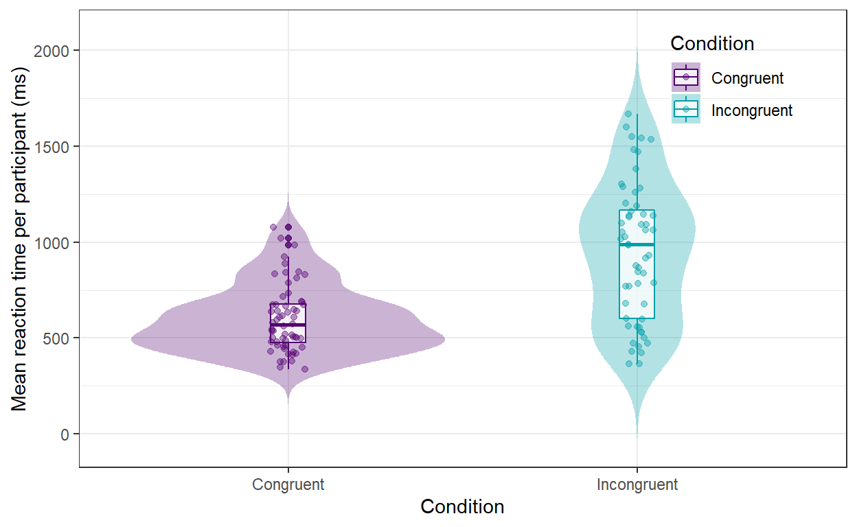
Visualise the distribution of mean reaction times per participants for each of the two groups.
stroop_clean %>%
  dplyr::rename(Condition = group) %>%
  ggplot2::ggplot(aes(x = Condition, y = m_rt, colour = Condition, fill = Condition)) +
  geom_violin(
    trim = FALSE,
    scale = "count",
    alpha = .3,
    color = NA
  ) +
  geom_boxplot(
    width = .1,
    fill="white", alpha = .8
  ) +
  geom_point(
    position = position_jitter(.05),
    alpha=.4) +
  labs(y = "Mean reaction time per participant (ms)") +
  scale_fill_manual(values = c("#52006f", "#009fa7")) +
  scale_colour_manual(values = c("#52006f", "#009fa7")) +
  theme_bw() +
  theme(legend.position = c(.85, .85),
        legend.background = element_blank())

Figure 1: Distribution of participants’ average reaction time (in ms) on valid colour-word trials by condition
Task 9
Create a well-formatted table of the following descriptive statistics per group:
- mean reaction time
- standard deciation of reaction time
- minimum and maximum of RT
- number of participants
desc_tib <- stroop_clean %>%
    dplyr::group_by(group) %>%
    dplyr::summarise(
      mean_rt = mean(m_rt),
      sd_rt = sd(m_rt),
      min = min(m_rt),
      max = max(m_rt),
      n = dplyr::n(),
      # we're going to need SE for plot of results
      se = sd_rt / sqrt(n)
    )
desc_tib %>%
  dplyr::select(-se) %>% # we don't need std. errors in our descriptive table
  kableExtra::kbl(
    digits = 1, # measurement is in grammes so we can just round to whole numbers
    col.names = c("Condition", "*M*", "*SD*", "Minimum", "Maximum", "*N*"),
    caption = "*Descriptive statistics of participants' average reaction time (in ms) on valid colour-word trials by condition.*") %>%
  kableExtra::kable_classic(full_width = FALSE)
| Condition | M | SD | Minimum | Maximum | N |
|---|---|---|---|---|---|
| Congruent | 600.3 | 174.4 | 335.3 | 1077.8 | 60 |
| Incongruent | 948.5 | 359.1 | 365.5 | 1669.5 | 56 |
The table should have informative column names and a caption.
Analysis
Task 10
Create an appropriate statistical model to test your hypothesis.
m1 <- t.test(m_rt ~ group, stroop_clean)
m1
    Welch Two Sample t-test

data:  m_rt by group
t = -6.5694, df = 78.329, p-value = 5.059e-09
alternative hypothesis: true difference in means between group Congruent and group Incongruent is not equal to 0
95 percent confidence interval:
 -453.7564 -242.7083
sample estimates:
  mean in group Congruent mean in group Incongruent
                 600.2761                  948.5085
Task 11
Report on any excluded data. How many observations did you exclude and for what reason?
We collected data from 116 participants, with 40 tirals per block, totalling 9280 observations. Of these, 411 were incorrect responses, 219 were non-responses, and 183 had improbably fast reaction times (< 200ms). These observation were excluded.
Task 12
Report the results in accordance with the APA guidelines.
Mean reaction time was, on average, shorter in the “Congruent” (600 ms, SD = 174 ms) than in the “Incongruent” condition (949 ms, SD = 359 ms). This difference was statistically significant according to Welch’s test, Mdiff = −348 ms, 95%CI [−454, −243], t(78.3) = −6.57, p < .001. We thus reject the null hypothesis of no difference in favour of the alternative.
Task 13
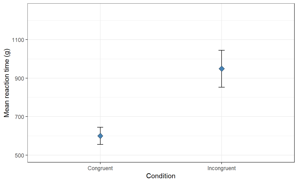
Visualise the results in a publication-quality errorbar plot.
- Plot should have a title and clearly labelled axes.
- It should be clear what the plot shows and what the errorbars represent.
desc_tib %>%
  dplyr::rename(Condition = group) %>%
  ggplot2::ggplot(aes(x = Condition, y = mean_rt)) +
  geom_errorbar(
    aes(
      ymin = mean_rt - 2 * se,
      ymax = mean_rt + 2 * se
    ),
    width = .05) +
  geom_point(
    shape = 23,
    size = 3,
    fill = "steelblue"
  ) +
  scale_y_continuous(
    name = "Mean reaction time (g)",
    limits = c(500, 1250) # custom limits to Y-axis
  ) +
  theme_bw()

Figure 2: Plot of mean reaction times on valid trials (±2×SE) by condition
Task 14
What do you conclude about your hypothesis based on your analysis?
We reject the null hypothesis of no difference in favour of the alternative.
Output
Task 15
Knit your .Rmd file into a formatted HTML document. Make sure it looks good and that there are no markdown rendering issues.
Well done!
If you successfully completed all the tasks, you’re ready to do the TAP.