In this tutorial, we will focus on strengthening your conceptual understanding of probability distributions, critical values, and proportions of the area below the curve. With the help of R will solve several problems in the context of the normal distribution, the t distribution, and the χ² distribution. However, bear in mind that the coding bit is of secondary interest here; what we want is to understand how the maths/code relates to different situations!

Setting up

All you need for this tutorial is this file, lecture 1 handout (link opens in new tab), and open RStudio. Just make sure you are working in the “week_03” R project created in your module folder to keep things well-organised. We won’t be needing to load any packages.

Lecture 1 quiz questions

To start off, let’s walk through the thinking needed to answer the questions in the “Test your understanding” sections of the handout.

Question 1

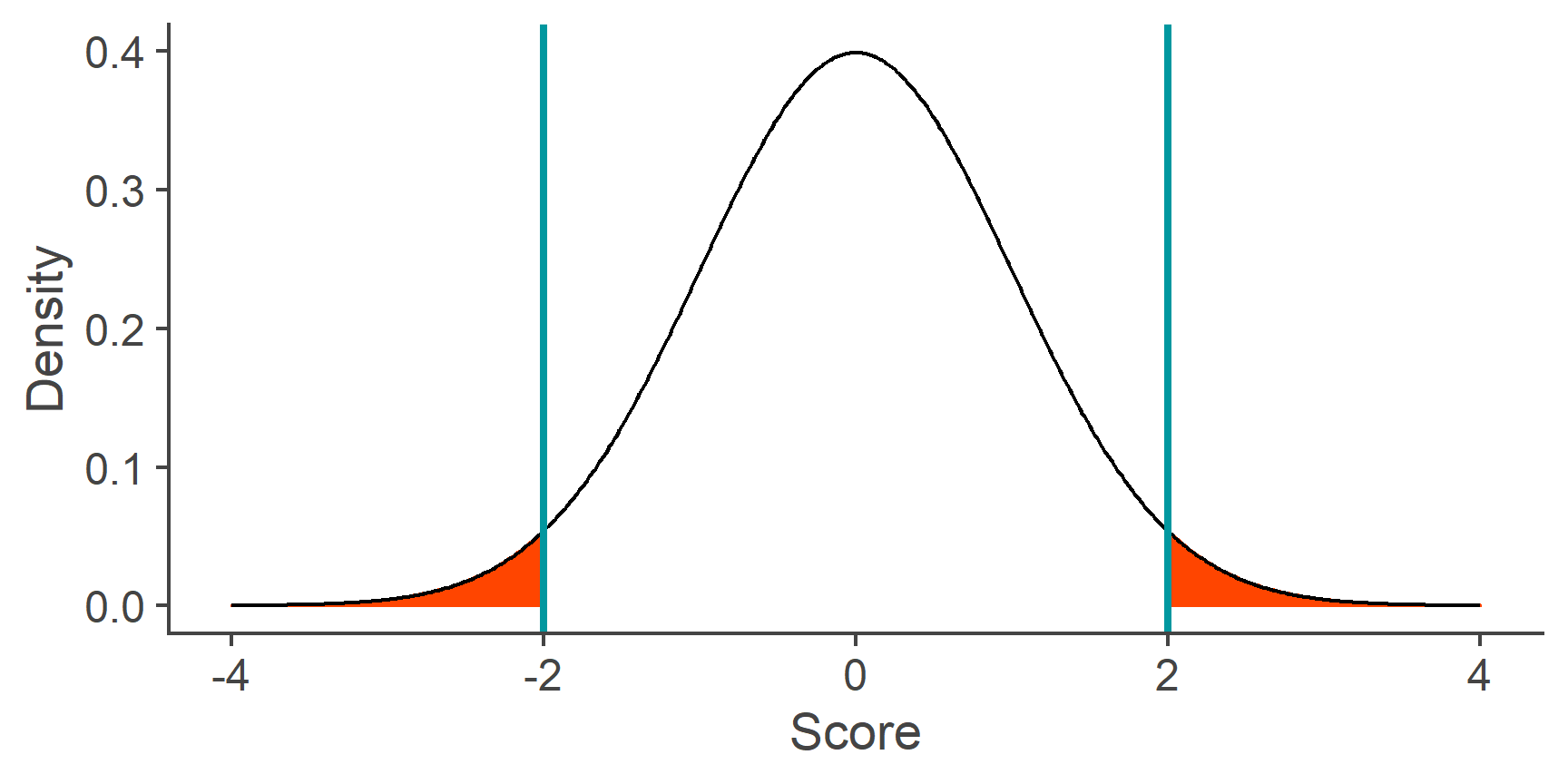
Both the lecture slides and the handout contain information about the percentage of the area below the standard normal curve that lie within ±2 SD from the mean. All we need to do then is realise that the question is only asking to do a single very simple operation – subtract this number from 100. This gives us the percentage of the curve that lies outside this cut–off point rather than inside.

Task 1

Correctly answer the first question in lecture 1 handout.

Question 2

In other words, this question asks us where do we need to draw the line along the x-axis in a normal distribution with a mean of 50 and a SD of 17.5, so that we cut it into two sections in a 30-70 ratio with respect to the area below the curve:

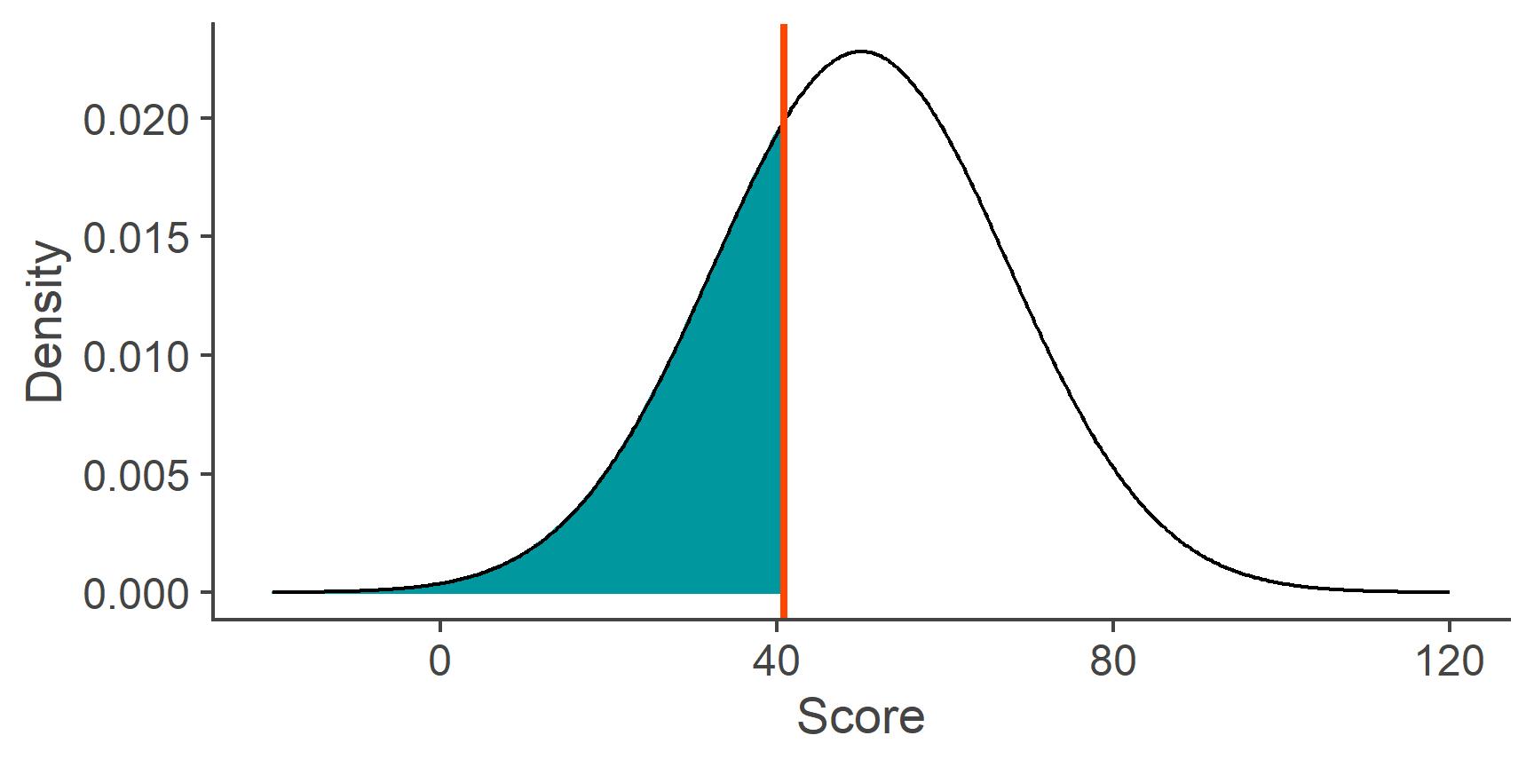
We need to realise that there are only 4 pieces of information that matter:

1. the distribution in question is normal,
2. its mean is 50,
3. its SD is 17.5,
4. and the quantile of interest cuts off 0.3 of the area below the curve counting from the left (lower) end.

Unless we’re good at maths and know how to integrate the normal function, we need to use R to get the question. Because the distribution we’re working with is normal, we’ll be using one of the *norm() functions. We know the mean and SD of the distribution and so we know what values we need to pass to the mean= and sd= arguments of the function. Since we know the probability/proportion we want to cut off (0.3) and want to know the quantile that cuts if off, rather than the other way around, we want to be using the qnorm() function, passing the value 0.3 to the first argument (p=). If the converse were the case and we wanted to know what proportion gets cut of by, let’s say, the score of 20 in this distribution, we’d be using the pnorm() function.

Task 2

Applying the above, what is the code that calculates the cut-off point?

qnorm(p = 0.3, mean = 50, sd = 17.5)

Task 3

Now that you know how to get the value, answer question 2 in the handout.

Question 3

This is basically the same question. All you need to answer it is to realise that 1.5% off the top is the same as 98.5% off the bottom and that a z-score is just the value of the x-axis in the standard normal distribution…

Task 4

Plug the right numbers into qnorm() to get the (unrounded) answer to question 3.

qnorm(p = 0.985)
# alternatively, you can get the qnorm function to give start from the top end
qnorm(p = 0.015, lower.tail = FALSE)

Question 4

Unlike the previous three questions, this one doesn’t call for the qnorm() function but for it’s inverse: pnorm(). Why? Because we want to know the probability of drawing a value equal to or larger than some IQ score. In other words, we want to know the proportion of the area below the curve from a given quantile to \(\infty\) in a normal distribution with the given values of \(\mu\) and \(\sigma\) (times 100 to get the percentage).

Task 5

Given the info above, correctly answer question 4.

Task 6

Without using R, what IQ score (from the same distribution as above) gives us the cut-off point for the lower 9.12%?

Task 7

Without using R, what score cuts off the top 9.12% of the normal distribution with a \(\mu\) of 0 and \(\sigma\) of 3?

Task 8

Without using R, what are the z-scores of the cut-off points in the previous 3 tasks?

Question 5

When solving these kinds of problems, the most important thing is to realise how the information in the question relates to the concepts that you need to apply. Here, the question is asking how many people out of 200, sampled at random from the normal distribution, would have z-scores less than −2 or more than 2.

This is just question 1 all over again but this time, you need to calculate how many people out of 200 corresponds to the answer to question 1.

Task 9

Ask R to calculate the answer to question 5 for you.

# proportion in the lower tail of the standard normal dist
lower_tail <- pnorm(-2)
# distribution is symmetrical so to get both tails, we multiply
prop <- lower_tail * 2
# get number of people
round(200 * prop)

[1] 9

So that’s the first set of questions out of the way and, hopefully, you are now more confident with the concepts of cut-off points and proportions of the are below the normal curve.

Let’s now have a look at the second set of questions. In order to answer them, we need to understand the concept of the sampling distribution as well as the relationships we talked about above.

n <- 20
mu <- 173
sigma <- 23

First of all, it’s important to keep in mind that all these questions are based around the same population distribution: a normal distribution with a \(\mu\) of 173 and \(\sigma\) of 23.

Questions 6 and 7

These questions are really rather straightforward provided you understand the sampling distribution of the mean. In the example given in the lecture handout, we were sampling bags of 20 apples. The sampling distribution is the distribution of all the sample means calculated on all possible such samples.

If you cannot see why both have the same answer, it might be a good idea to spend more time reading up on the sampling distribution. In fact, it is highly recommended.

Question 8

Once you unpack this question, it’s quite easy. The range of sample means we can expect is dependent on the magnitude of SE, the standard deviation of the sampling distribution. Because the sampling distribution is normal, we can easily find the critical value – the multiple of SD – that cuts off bottom and top 2.5% of it’s area:

qnorm(c(.025, .975))

[1] -1.959964  1.959964

All we need to do now is to find the mean of the sampling distribution and the SE. We know the mean of the sampling distribution (see questions 6 and 7) and SE is easily calculated using the formula:

\[SE = \frac{\sigma}{\sqrt{N}}\] Once you plug in the numbers, you’ll get the answer. The range of sample means we can expect with a 95% probability is just the range formed by \(\mu \pm 1.96\times SE\)

# mean of samp dist of the mean is the same as mu
mu <- 173
# critical values for inner 95% of normal dist
crit_vals <- qnorm(c(.025, .975))
# std error
se <- 23 / sqrt(20)

# inner 95% of the sampling dist = range of means
mu + crit_vals * se

[1] 162.92 183.08

# alternatively we can plug mu and se into qnorm
qnorm(c(.025, .975), mean = mu, sd = se)

[1] 162.92 183.08

Question 9

This is the same question, just based on the sampling distribution of the mean when N = 50. This change affects only one of the values we use in the calculation.

Task 10

Calculate the answer to question 9 without further help.

Question 10

Based on what we talked about in question 8, this should be a very simple calculation…

23 / sqrt(100)

[1] 2.3

The last three questions demonstrate the relationship between sample size, standard error, and the spread of the sampling distribution. Given a fixed value of population standard deviation, the smaller the sample, the more the individual sample means will vary. That’s because it’s easier to get a really unusual sample (for example very small apples) when we’re only picking 5 observations than it is if we’re picking 100.

Other distributions

Grasping the concept of area under a curve and critical values as scores on the x-axis that cut off an arbitrary proportion of this area is crucial for understanding statistical testing. Different statistical tests work with different distributions but the principle behind critical values is the same, no matter the distribution we are looking at. There is one notable difference, however: While any normal distribution can always be transformed into the standard normal (mean = 0, SD = 1) so that the standard critical values can be applied, this is not the case with other distributions. As discussed in lecture 2, there are distributions whose shape changes as a function of some parameter. And with their shape, the critical values for any given proportion of the are under the curve change as well.

Let’s have a look at two of these distributions.

The t distribution

We talked about the t distribution (AKA Student’s¹ t distribution) in lecture 2, where we learnt how we can use it to approximate the sampling distribution of the mean when we don’t know the true standard error.

The t distribution is symmetrical, fairly bell-shaped, and always centred around zero. Unlike the normal distribution, it is not characterised by its mean and SD but by the number of degrees of freedom (df).

Have a little play around with the visualisation below. It shows you how the critical values that cut off the outer 5% tails change as a function of the number of dfs.

As you can see, there is are R function equivalents of pnorm() and qnorm() for the t distribution: pt() and qt(), respectively.

Task 11

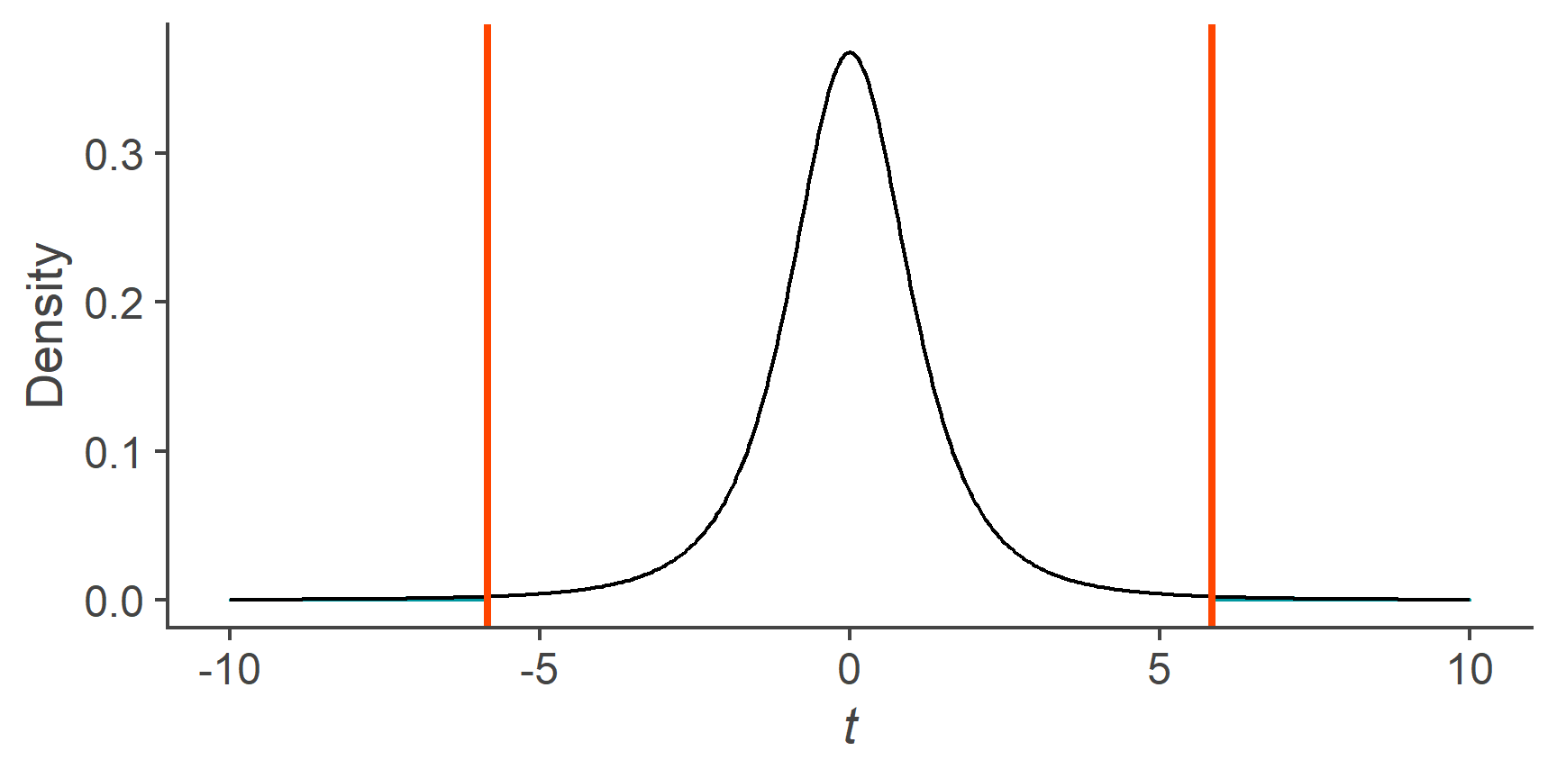
Calculate the critical values that cut off the most extreme 1% of the area below the curve of a t distribution with 3 df.

qt(p = c(.005, .995), df = 3)

[1] -5.840909  5.840909

Task 12

Calculate the critical value that cuts off the upper 5% of the area below the curve of a t distribution with 25 df.

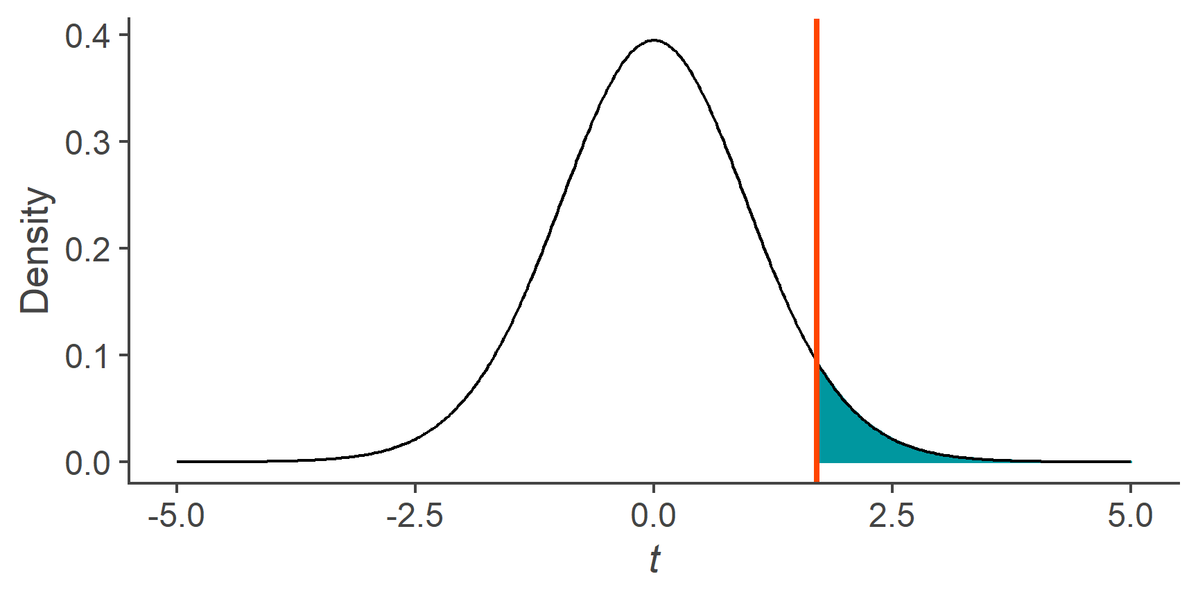
qt(p = .95, df = 25)

[1] 1.708141

Task 13

Calculate the probability of randomly sampling a point from a t distribution with 100 df, whose value is smaller than 1.5.

pt(q = 1.5, df = 100)

[1] 0.9316175

The \(\chi^2\) distribution

Finally, let’s transfer what we know to a context of a distribution we have not talked about yet, just to illustrate that it’s all just the same thing.

The \(\chi^2\) distribution (pronounced /kai/-squared) is a little different from the normal and t distributions in that it is not symmetrical. It ranges from 0 to \(\infty\) and, just like the t distribution, its shape changes as a function of degrees of freedom.

Have a go at the applet below to see that the proportions of the \(\chi^2\) distribution (and with them, the critical values) change rather dramatically with different number of df.

And just like before, we can use the qchisq() and pchisq() functions to calculate critical values, given some probability and vice versa, respectively.

Task 14

Calculate the critical value that cuts off the upper 5% of the area below the curve of a \(\chi^2\) distribution with 25 df.

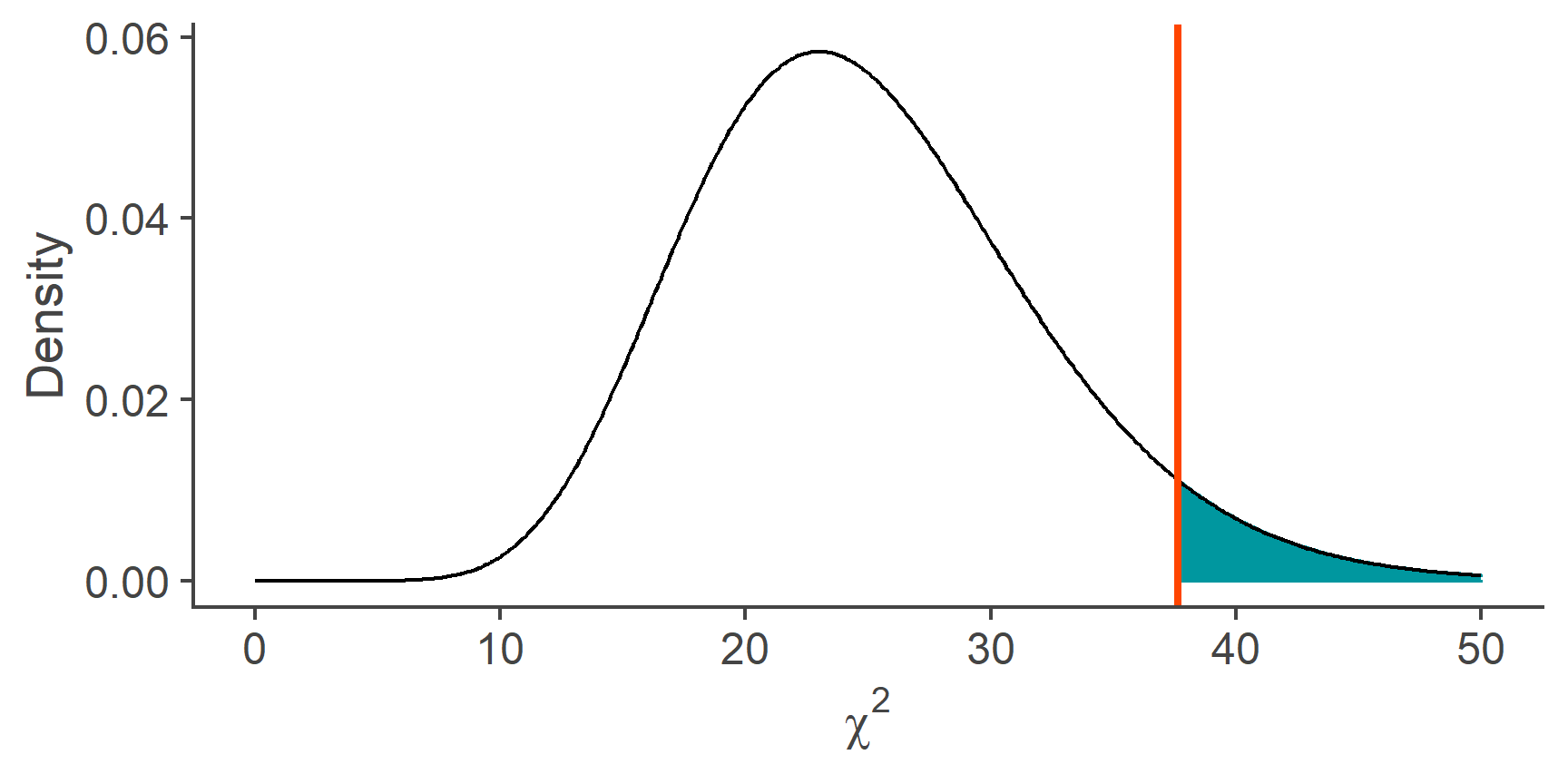
 qchisq(p = .95, df = 25)

[1] 37.65248

Task 15

Calculate the probability of getting randomly sampling a value from a \(\chi^2\) distribution with 4 df, that’s at least 11.5.

pchisq(q = 11.5, df = 4, lower.tail = FALSE)

[1] 0.02148377

By the way, the \(\chi^2\) distribution is the sampling distribution of the variance (with df = N − 1). If you think about it, variance can never be less than 0 which is why the distribution is only defined for non-negative numbers.

That’s all for now.