Setting Up
Task 1
Open your project for this week in RStudio. Then, open a new Markdown file with HTML output and save it in the r_docs folder. (Give it a sensible name, like worksheet_09 or similar!)
For each of the tasks in the Analysis section, write your code to complete the task in a new code chunk.
Remember, you can add new code chunks by:
- Using the RStudio toolbar: Click Code > Insert Chunk
- Using a keyboard shortcut: the default is Ctrl + Alt + I (Windows) or ⌘ Command + Option + I (MacOS), but you can change this under Tools > Modify Keyboard Shortcuts…
- Typing it out:
```{r}, press ↵ Enter, then```again. - Copy and pasting a code chunk you already have (but be careful of duplicated chunk names!)
I Wanna Be the Very Best
The theme for today’s task is inspired by a weird Internet thing that happened in the spring of 2014, called Twitch Plays Pokémon. A programmer in Australia hooked up the classic Pokémon Red game to the chat room on video game streaming site Twitch. By typing commands in the chat, viewers could control what the character in the game did - but on the scale of thousands or tens of thousands of participants at once. The game turned into a massive social experiment and even spawned a minor cult before the cumulative 1.16 million viewers beat the game in about two and a half weeks1.
To Catch Them Is My Real Test, To Train Them Is My Cause
If you aren’t really familiar with Pokémon, all you need to know for today is that it’s a series of video games (later TV show, graphic novels, etc. etc.) that take place in an alternate universe with magical animals called Pokémon. Pokémon battling (sort of like magical dogfighting?) is a core part of this universe, with children setting out at a young age to travel the world, capture many different types of Pokémon, and compete in massive championships, with the winner being crowned a Pokémon Master. It’s a bit ethically murky because at least some Pokémon seem to be sentient, and they can all talk, but only to say their own species name. You know, as I’m writing this description, it just keeps sounding weirder…
 Figure 1 A Pokémon called Pikachu. You may have heard of him. Source
For this week’s stats practical, we’re doing a Twitch-Plays-Pokémon-style walkthrough of a dataset of Pokémon characteristics to practice the linear model. You don’t need to know anything about Pokémon to do this practical besides what’s in the box above.
Task 2
Load the tidyverse package and read in the pokemon dataset straight from https://and.netlify.app/datasets/pokemon.csv (we took the data from this fun website).
Task 3
You should always have a look at what variables you have in your data. Do it now by asking R to either give you the names of the variables or by looking at a rought summary of the data.
As you can see there are quite a few variables but most of them will not be relevant to us.
Making Predictions
First we need to choose a research question to investigate.
As future Pokémon Masters, we want to work out which Pokémon is the strongest. So, we’ll use attack as our outcome variable, which quantifies a Pokémon’s offensive capabilities.
For the predictor, let’s choose the hp variable.
HP or hit points is a geek gaming term name for health of your character/creature:
The more HP a thing has, the more damage it can withstand.
Task 4
In your RMarkdown file, write down your prediction about the relationship between the predictor – hp – and the outcome, attack.
Visualising the Relationship
Next up, we should have a look at our data.
Task 5
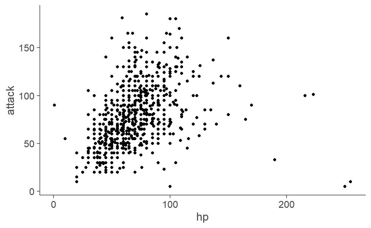
Create a scatterplot of hp as the predictor and attack as the outcome.
pokemon %>%
  ggplot(aes(x = hp, y = attack)) +
  geom_point()
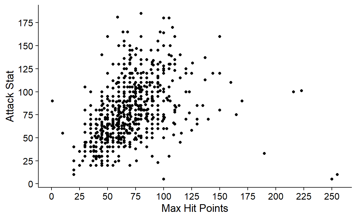
Task 5.1
Label the axes better and clean up the plot with a theme.
pokemon %>%
  ggplot(aes(x = hp, y = attack)) +
  geom_point() +
  scale_x_continuous(name = "Max Hit Points",
                     # seq() creates a vector of breaks at increments of 25
                     breaks = seq(0, max(pokemon$hp), by = 25)) +
  scale_y_continuous(name = "Attack Stat",
                     breaks = seq(0, max(pokemon$attack), by = 25)) +
  cowplot::theme_cowplot()
Task 5.2
Stop and have a look at your plot. How would you draw the line of best fit? Is this the direction of relationship you expected?
Task 5.3
Add a line of best fit to your plot. Is this what you expected?
pokemon %>%
  ggplot(aes(x = hp, y = attack)) +
  geom_point() +
  scale_x_continuous(name = "Max Hit Points",
                     # seq() creates a vector of breaks at increments of 25
                     breaks = seq(0, max(pokemon$hp), by = 25)) +
  scale_y_continuous(name = "Attack Stat",
                     breaks = seq(0, max(pokemon$attack), by = 25)) +
  geom_smooth(method = "lm") +
  cowplot::theme_cowplot()

Task 5.4
Optionally, add another line to your plot that represents the null model.
Have a look at geom_hline, or the code for the plots in the lecture!
pokemon %>%
  ggplot(aes(x = hp, y = attack)) +
  geom_point() +
  scale_x_continuous(name = "Max Hit Points",
                     breaks = seq(0, max(pokemon$hp), by = 25)) +
  scale_y_continuous(name = "Attack Stat",
                     breaks = seq(0, max(pokemon$attack), by = 25)) +
  geom_hline(yintercept = mean(pokemon$attack), linetype = "dashed") +
  geom_smooth(method = "lm") +
  cowplot::theme_cowplot()

Creating the Model
Now that we have some idea of what to expect, we can create our linear model!
Task 6
Use the lm() function to run your analysis and save the model in a new object called poke_lm.
# remember to use whichever predictor you've chosen!
poke_lm <- lm(attack ~ hp, data = pokemon)
Task 7
Call this poke_lm object in the Console to view it, then write out the linear model from the output.
First, to see what’s in our model, we can just call it by typing its name in the console and pressing Enter.
poke_lm
Call:
lm(formula = attack ~ hp, data = pokemon)

Coefficients:
(Intercept)           hp
    43.5939       0.4969
As we’ve seen before, this simple version of the output gives us two numbers:
(Intercept): the intercept, here 43.59hp: the slope, here 0.5
Keep in mind that the slope will always be named with the predictor that it’s associated with!
So, we can write our linear model: \(\text{Attack}_i = 43.59 + 0.5 \times \text{HP}_i\).
Task 8
How can you interpret the value of b1 for this model? Write down your thoughts in your RMarkdown.
For the hp predictor, the value of b1 is 0.5. This is the predicted change in attack for each unit change in hp. In other words, for each additional hit point a Pokémon has, it’s predicted to have 0.5 more hit points - a positive relationship.
Task 9
Using your equation, what attack value would you predict a Pokémon with 86 HP to have?
Start with our equation: \(\text{Attack}_i = 43.59 + 0.5 \times \text{HP}_i\).
All we need to do is replace the value of HP with the specific value we’re interested in:
\[\begin{aligned}\text{Attack} &= 43.59 + 0.5 \times 86\\ &= 43.59 + 43\\ &= 86.59\end{aligned}\]
Weirdly enough (and completely coincidentally), a Pokémon with 86 HP should have an attack rating of about 86!
Evaluating the Model
Now we have the model parameters, but we don’t want to just describe the line - we want to be able to say something about the population, not just our sample. For this, we need some more info!
Significance Testing
Task 10
Use broom::tidy() to get p-values for your bs. Is your predictor significant?
Remember, that in the so-called scientific notation, the number xe-n, where x and n are numbers means x × 10−n.
For example 2.3e-4 means 2.3 × 10⁻⁴ which is the same as 2.3/10000 or 0.00023.
# A tibble: 2 x 5
  term        estimate std.error statistic  p.value
  <chr>          <dbl>     <dbl>     <dbl>    <dbl>
1 (Intercept)   43.6      2.88        15.1 1.41e-45
2 hp             0.497    0.0390      12.7 6.27e-34
Yikes, look at those p-values! That’s a lot of 0s. I think we can safely say that both these values are smaller than .05, although the one we really care about here is for the predictor, hp.
Task 11
Add the conf.int = T argument to broom::tidy() to get confidence intervals. How can you interpret these? Do they “agree” with the p-value?
# A tibble: 2 x 7
  term        estimate std.error statistic  p.value conf.low conf.high
  <chr>          <dbl>     <dbl>     <dbl>    <dbl>    <dbl>     <dbl>
1 (Intercept)   43.6      2.88        15.1 1.41e-45   37.9      49.3
2 hp             0.497    0.0390      12.7 6.27e-34    0.420     0.573
Again, we’re mainly interested in b1, which is hp. First we want to know if these confidence intervals cross or include 0. Looking at these two values, neither of them are exactly 0, and both values are positive. So, they don’t cross or include 0.
Remember that the confidence intervals give us a range of likely values of b1 from other samples. If the confidence intervals don’t cross or include 0, as we can see here, it’s unlikely that we could have gathered a sample where b1 was 0. This “agrees” with our p-value, which indicated that the probability of obtaining the results we have, assuming the null hypothesis is true, is very very small. Altogether the evidence suggests that it’s quite unlikely that the relationship between HP and attack is actually 0 (no relationship at all).
Goodness of Fit
Task 12
Use broom::glance() to get R2 and adjusted R2 for this model.
How much of the variance of the outcome is explained by the model for this sample? What would we expect this to be in the population?
# A tibble: 1 x 12
  r.squared adj.r.squared sigma statistic  p.value    df logLik   AIC
      <dbl>         <dbl> <dbl>     <dbl>    <dbl> <dbl>  <dbl> <dbl>
1     0.169         0.168  29.3      162. 6.27e-34     1 -3842. 7690.
# ... with 4 more variables: BIC <dbl>, deviance <dbl>,
#   df.residual <int>, nobs <int>
For now we can ignore everything in this output except for the values labeled r.squared and adj.r.squared.
To answer the questions, we can simply convert them to percentages by multiplying by 100.
Variance in the outcome explained by the model in the sample: 16.86%
Estimated variance in the outcome explained by the model in the population: 16.76%
Reading the Summary
Finally, we can get all this same information - except for CIs - from the summary() function.
I (Jennifer) like summary() because you can get a good overview of a lot of information quickly, but it’s very inconvenient for reporting, so it’s good to know how to use the broom functions as well.
Task 13
Get a summary of your model. What do the asterisks (stars) mean?
Call:
lm(formula = attack ~ hp, data = pokemon)

Residuals:
     Min       1Q   Median       3Q      Max
-162.812  -18.469   -3.344   16.656  108.091

Coefficients:
            Estimate Std. Error t value Pr(>|t|)
(Intercept) 43.59387    2.88447   15.11   <2e-16 ***
hp           0.49687    0.03903   12.73   <2e-16 ***
---
Signif. codes:  0 '***' 0.001 '**' 0.01 '*' 0.05 '.' 0.1 ' ' 1

Residual standard error: 29.34 on 799 degrees of freedom
Multiple R-squared:  0.1686,    Adjusted R-squared:  0.1676
F-statistic:   162 on 1 and 799 DF,  p-value: < 2.2e-16
We can see all of the same numbers here that we saw before, even labeled the same way.
summary() also gives us the stars at the end of each line, which give us an idea of what alpha level each element of the model is significant at.
As you can see, our predictor has three stars, which corresponds to p < .001.
Reporting
Task 14
Report the results of your model. Specifically, you should clearly report the coefficient of interest (b1) and the fit of the model (R2), including all the important details (see Tutorial 8).
You can read all the important information from the summary() and of your model type them up manually but you can also use the apa_print() function from the papaja package.
To do that, let’s first see what the function returns:
papaja::apa_print(poke_lm)
$estimate
$estimate$Intercept
[1] "$b = 43.59$, 95\\% CI $[37.93$, $49.26]$"

$estimate$hp
[1] "$b = 0.50$, 95\\% CI $[0.42$, $0.57]$"

$estimate$modelfit
$estimate$modelfit$r2
[1] "$R^2 = .17$"

$estimate$modelfit$r2_adj
[1] "$R^2_{adj} = .17$"

$estimate$modelfit$aic
[1] "$\\mathrm{AIC} = 7,690.27$"

$estimate$modelfit$bic
[1] "$\\mathrm{BIC} = 7,704.33$"


$statistic
$statistic$Intercept
[1] "$t(799) = 15.11$, $p < .001$"

$statistic$hp
[1] "$t(799) = 12.73$, $p < .001$"

$statistic$modelfit
$statistic$modelfit$r2
[1] "$F(1, 799) = 162.04$, $p < .001$"


$full_result
$full_result$Intercept
[1] "$b = 43.59$, 95\\% CI $[37.93$, $49.26]$, $t(799) = 15.11$, $p < .001$"

$full_result$hp
[1] "$b = 0.50$, 95\\% CI $[0.42$, $0.57]$, $t(799) = 12.73$, $p < .001$"

$full_result$modelfit
$full_result$modelfit$r2
[1] "$R^2 = .17$, $F(1, 799) = 162.04$, $p < .001$"


$table
A data.frame with 5 labelled columns:

  predictor estimate                 ci statistic p.value
1 Intercept    43.59 $[37.93$, $49.26]$     15.11  < .001
2        Hp     0.50   $[0.42$, $0.57]$     12.73  < .001

predictor: Predictor
estimate : $b$
ci       : 95\% CI
statistic: $t(799)$
p.value  : $p$
attr(,"class")
[1] "apa_results" "list"
As you can see, the returned list contains quite a lot of stuff:
- The
estimateelement contains, among other things your b and R2 coefficients along with their respective 95% and 90% CIs, respectively. The reason why R2 is reported with a 90% rather than a 95% CI is not really important right now. - The
statisticelement contains the results of the statistical tests of the individual coefficients (t and p-values) and the overall model fit (F-test, which we haven’t covered yet). - The
full_resultselement contains the two combined. - Finally, the
tableelement contains the data we can use to easily create a basic table of model results.
To ask for the individual elements, we should first save the output of the function in the environment by assigning it to a name:
res <- papaja::apa_print(poke_lm)
We can now use the dollar sign notation to ask for individual elements.
Let’s see what the full_result one gives us:
res$full_result
$Intercept
[1] "$b = 43.59$, 95\\% CI $[37.93$, $49.26]$, $t(799) = 15.11$, $p < .001$"

$hp
[1] "$b = 0.50$, 95\\% CI $[0.42$, $0.57]$, $t(799) = 12.73$, $p < .001$"

$modelfit
$modelfit$r2
[1] "$R^2 = .17$, $F(1, 799) = 162.04$, $p < .001$"
The outcome is again a list we can further query using $:
# report full results for slope of HP
res$full_result$hp
[1] "$b = 0.50$, 95\\% CI $[0.42$, $0.57]$, $t(799) = 12.73$, $p < .001$"# report model fit
res$full_result$modelfit$r2
[1] "$R^2 = .17$, $F(1, 799) = 162.04$, $p < .001$"To report the results in the body of our report/paper/dissertation, we would say something like:
The model accounted for a significant proportion of variance in the ouctome, \(R^2 = .17\), \(F(1, 799) = 162.04\), \(p < .001\). The number of hit points of a Pokémon was a significant predictor of its attack strength, \(b = 0.50\), 95% CI \([0.42\), \(0.57]\), \(t(799) = 12.73\), \(p < .001\). These results support our hypothesis.
You can also easily report the results in a nice table:
# <br> in caption is a line break
res$table %>%
  kableExtra::kbl(
    col.names = c("Predictor", "*b*", "95% CI", "*t*(799)", "*p*"),
    caption = "Table 1<br>*Results of the linear model predicting attack strength by the number of hit points.*"
  ) %>%
  kableExtra::kable_classic(full_width=FALSE)
| Predictor | b | 95% CI | t(799) | p |
|---|---|---|---|---|
| Intercept | 43.59 | \([37.93\), \(49.26]\) | 15.11 | < .001 |
| Hp | 0.50 | \([0.42\), \(0.57]\) | 12.73 | < .001 |
I Know It’s My Destiny
That’s as far as we’ll go today, well done!
The Linear Model is all of our destinies for the next year or so, so it’s important to get comfortable working with it.
I (Jennifer) was doing my first year of PhD in Edinburgh, actually sat at the desk next to* our own Milan Valášek (the universe is weird like that!). Because I spent a lot of my time on the Internet instead of, y’know, doing my work, I watched a lot of this unfold in real time. It was even stranger than this makes it sound.
*Actually, she kind of sat right behind my back which was rather unnerving. ~Milan↩︎